If you aren't familiar with Streaming Expressions new statistical programming functions you may find it useful to read a few of the earlier blogs which introduce the topic.
- Statistical programming with Solr Streaming Expressions
- One-way ANOVA and Rank Transformation with Solr's Streaming Expressions
- A first look at Sunplot, a statistical plotting engine for Solr Streaming Expressions
- Detrending Time Series Data With Linear Regression in Solr 7
- Time Series Cross-correlation and Lagged Regression With Solr Streaming Expressions
Seasonality
Often seasonality appears in the data as periodic bumps or waves. These waves can be expressed as sine-waves. For this example we'll start off by generating some smooth sine-waves to represent seasonality. We'll be using Solr's statistical functions to generate the data and Sunplot to plot the sine-waves.
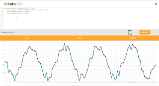
Here is a sample plot using Sunplot:
In the plot you'll notice there are waves in the data occurring at regular intervals. These waves represent the seasonality.
The expression used to generate the sine-waves is:
let(smooth=sin(sequence(100, 0, 6)),
plot(type=line, y=smooth))
In the function above the let expression is setting a single variable called smooth. The value set to smooth is an array of numbers generated by the sequence function that is wrapped and transformed by the sin function.
Then the let function runs the plot function with the smooth variable as the y axis. Sunplot then plots the data.
This sine-wave is perfectly smooth so the entire time series consists only of seasonality. To make things more interesting we can add some noise to the sign-waves to represent another component of the time series.
Now the expression looks like this:
let(smooth=sin(sequence(100, 0, 6)),
noise=sample(uniformDistribution(-.25,.25),100),
noisy=ebeAdd(smooth, noise),
plot(type=line, y=noisy))
In the expression above we first generate the smooth sine-wave and set it to the variable smooth. Then we generate some random noise by taking a sample from a uniform distribution. The random samples will be uniformly distributed between -.25 and .25. The variable noise holds the array of random noise data.
Then the smooth and noise arrays are added together using the ebeAdd function. The ebeAdd function does an element-by-element addition of the two arrays and outputs an array with the results. This will add the noise to the sine-wave. The variable noisy holds this new noisy array of data.
The noisy array is then set to the y axis of the plot.
Now we have a time series that has both a seasonality component and noisy signal. Let's see how we can model and remove the seasonality so we can study the noisy component.
Modeling Seasonality
We can model the seasonality using the new polyfit function to fit a curve to the data. The polyfit function is a polynomial curve fitter which builds a function that models non-linear data.
Below is a screenshot of the polyfit function:
Notice that now there is a smooth red curve which models the noisy time series. This is the smooth curve that the polyfit function fit to the noisy time series.
Here is the expression:
let(smooth=sin(sequence(100, 0, 6)),
noise=sample(uniformDistribution(-.25,.25),100),
noisy=ebeAdd(smooth,noise),
fit=polyfit(noisy, 16),
x=sequence(100,0,1),
list(tuple(plot=line, x=x, y=noisy),
tuple(plot=line, x=x, y=fit)))
In the expression above we first build the noisy time series. Then the polyfit function is called on the noisy array with a polynomial degree. The degree describes the exponent size of the polynomial used in the curve fitting function. As the degree rises the function has more flexibility in the curves that it can model. For example a degree of 1 provides a linear model. You can try different degrees until you find the one that best fits your data set. In this example a 16 degree polynomial is used to fit the sine-wave.
Notice that when plotting two lines we use a slightly different plotting syntax. In the syntax above a list of output tuples is used to define the plot for Sunplot. When plotting two plots an x axis must be provided. The sequence function is used to generate an x axis.
Removing the Seasonality
Once we've fit a curve to the time series we can subtract it away to remove the seasonality. After the subtraction what's left is the noisy signal that we want to study.
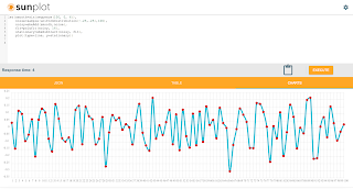
Below is a screenshot showing the subtraction of the fitted curve:
Notice that the plot now shows the data that remains after the seasonality has been removed. This time series is now ready to be studied without the effects of the seasonality.
Here is the expressions:
let(smooth=sin(sequence(100, 0, 6)),
noise=sample(uniformDistribution(-.25,.25),100),
noisy=ebeAdd(smooth,noise),
fit=polyfit(noisy, 16),
stationary=ebeSubtract(noisy, fit),
plot(type=line, y=stationary))
In the expression above the fit array, which holds the fitted curve, is subtracted from the noisy array. The ebeSubtract function performs the element-by-element subtraction. The new time series with the seasonality removed is stored in the stationary variable and plotted on the y axis.


